필사 모드: AI for Everyone, Part 5 — Colourising Photos With a 0.47M U-Net, and Why the Colours Came Out Washed Out
English- When the output is an image
- U-Net — what skip connections carry
- Training
- Results — shapes right, colours drained
- Why the colours drained — the nature of L1
- What real colourisation models do
- Summary
- 🧠 Comprehension quiz
- References
When the output is an image
So far the output has been text: sentences in Part 1, words in Part 3, captions in Part 4. This time the output is an image itself.
The task is colourisation. Feed in a greyscale photo, get a colour one back.
input:  32x32 greyscale (1 channel)
output: 32x32 colour    (3 channels)
No separate dataset is needed. Convert CIFAR-10's colour images to greyscale and the input-target pairs create themselves.
rgb = torch.stack([...])                                    # original colour = target
gray = (rgb * torch.tensor([0.299, 0.587, 0.114])
        [None, :, None, None]).sum(1, keepdim=True)         # greyscale = input
The weights 0.299, 0.587, 0.114 are the standard luminance formula, reflecting that human eyes are most sensitive to green and least to blue. Data built this way is called self-supervised: nobody labelled anything, yet targets exist.
U-Net — what skip connections carry
Colourisation has an awkward requirement. You must know what something is to pick its colour, but you must also know exactly where it is. Recognising a frog tells you to paint green; letting that green bleed past the frog's outline ruins it.
A plain encoder-decoder struggles with both at once, because compressing the image gains meaning while losing position. U-Net resolves this with skip connections.
class TinyUNet(nn.Module):
    def __init__(self):
        super().__init__()
        self.e1 = block(1, 32); self.e2 = block(32, 64); self.e3 = block(64, 128)
        self.d2 = block(128 + 64, 64); self.d1 = block(64 + 32, 32)
        self.out = nn.Conv2d(32, 3, 1)

    def forward(self, x):
        s1 = self.e1(x)                       # 32x32  — finest detail
        s2 = self.e2(F.max_pool2d(s1, 2))     # 16x16
        h  = self.e3(F.max_pool2d(s2, 2))     # 8x8    — most abstract
        h = self.d2(torch.cat([F.interpolate(h, scale_factor=2), s2], 1))
        h = self.d1(torch.cat([F.interpolate(h, scale_factor=2), s1], 1))
        return torch.sigmoid(self.out(h))
The key is torch.cat([upsampled_h, s2], 1). As the decoder restores resolution, it pulls in the encoder output at the matching resolution and concatenates it.
h, arriving from below — low resolution, but carrying meaning like "this is a frog"s2, arriving from the side — never compressed, so edges and texture are intact
The decoder sees both. Meaning comes from the deep path, position from the skip path. That is why the channel count reads 128 + 64.
Ending with sigmoid is also deliberate: the output must be RGB in the 0–1 range, so the activation enforces it.
Training
opt = torch.optim.AdamW(model.parameters(), lr=2e-3)

while not run.over_budget():          # 12-minute budget
    ix = torch.randint(0, len(rgb), (128,))
    x, y = gray[ix].to(dev), rgb[ix].to(dev)
    loss = F.l1_loss(model(x), y)
    opt.zero_grad(); loss.backward(); opt.step()
The loss is L1 (mean absolute error) — a regression loss measuring the raw difference between predicted and true RGB values. This choice determines the character of the result, as we will see.
[   14.1s] pairs=30000
[   14.2s] params {"params": 472323, "res": 32}
[  722.0s] SUMMARY {"steps": 62136, "final_l1": 0.0231}
62,136 steps, final L1 of 0.023. With pixel values in 0–1, that is a 2.3% average error. By the numbers alone, excellent.
Results — shapes right, colours drained
Each row holds two groups of three, ordered input greyscale / model prediction / true colour.
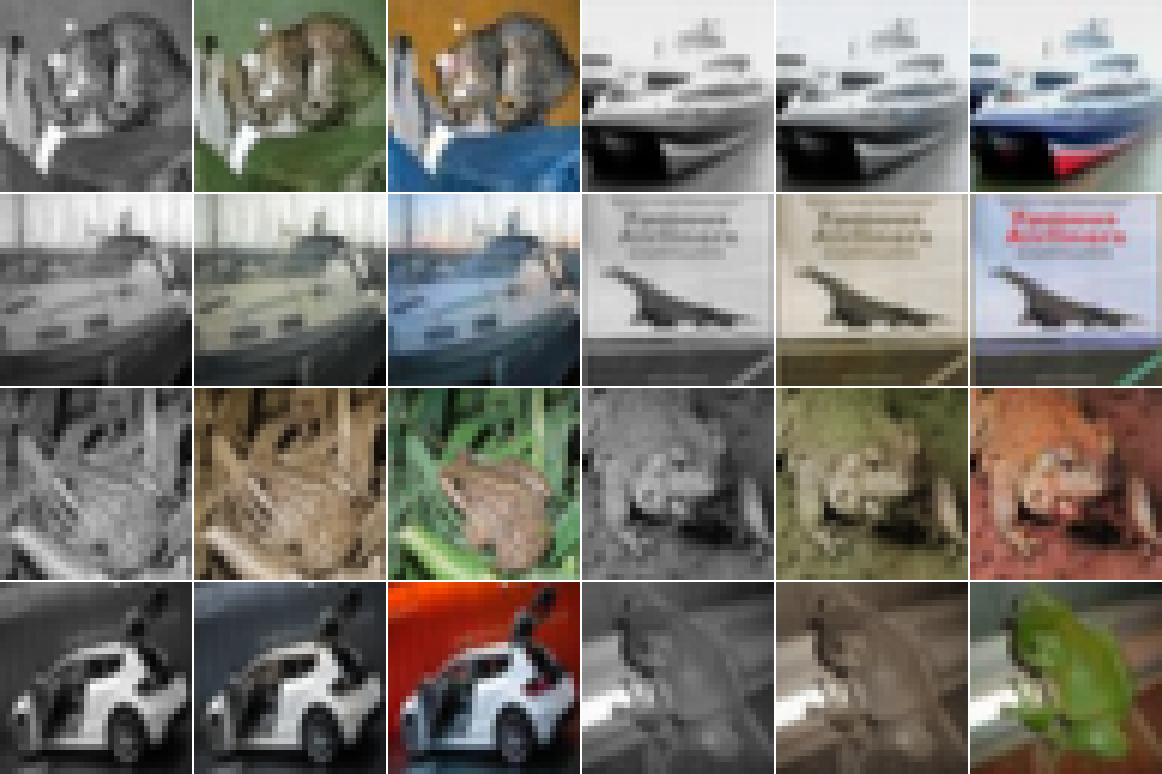
Read honestly.
What works — shapes are preserved exactly. Cat fur, the ship's deck structure, the frog's legs, the car's window frames are all crisp. That is skip connections doing their job. The direction of colour is mostly right too: green around the frog, blue around the ship, brownish for the cat.
What does not — the colours are washed out. A car that is vivid red in the target comes back dark grey-brown. A red hull and blue sea become murky grey-blue. Many results sit close to sepia.
Why the colours drained — the nature of L1
This is not because the model is small. It is a consequence of choosing L1.
Consider one greyscale photo of a car. That car could be red, blue, or white. Greyscale alone cannot settle it. In other words, this is a problem with many valid answers.
L1 tells the model: minimise the absolute error against the target. When several answers are possible, what is the safest way to obey?
Predict the middle of all possibilities.
Guess red and get blue, and the penalty is severe. Guess grey and the penalty stays moderate whatever the truth turns out to be. As training proceeds the model converges on that safe strategy, and the product of it is desaturated colour.
That is how a good L1 of 0.023 and washed-out colour coexist. L1 did exactly what it was asked to do; what it was asked was not what we wanted.
What real colourisation models do
The problem is well known, and the fixes fall into a few families.
Turn colour into classification — Zhang et al. (2016) divided the colour space into 313 bins and asked which bin each pixel belongs to. Classification lets probability be spread across several candidates, so nothing gets averaged away; you then sample a vivid one.
Add an adversarial loss — a GAN discriminator asks whether an image looks real. Washed-out colour does not look like a real photograph, so it gets penalised. L1 handles shape, the discriminator handles vividness.
Use a perceptual loss — compare in the feature space of a pretrained network rather than comparing pixel values, which is closer to how people judge similarity.
All three share one idea: design the loss so that fleeing to the average stops paying off.
Summary
| Item | Value |
|---|---|
| Parameters | 472,323 (0.47M) — smallest in the series |
| Training time | 722.0s |
| Steps | 62,136 |
| Final L1 | 0.0231 |
| Data | 30,000 CIFAR-10 pairs (self-supervised) |
With 472 thousand parameters, colour was applied while shape stayed intact. Skip connections kept fine structure alive, and the self-supervised setup cost nothing to label.
The real lesson, though, sits on the washed-out side. A loss function defines the goal; it is not a tool for reaching one. The moment L1 was chosen, the rule "answers near the average are safe" came with it, and the model followed that rule faithfully. If the result disappoints, the first thing to revisit is not the model but what you told it to minimise.
The next part takes this problem head-on with diffusion — a structure that picks one answer instead of fleeing to the average when many answers are possible.
🧠 Comprehension quiz
1. How would the colourisation change without skip connections?
Shapes would blur. Compressing to 8×8 destroys edge and texture information, and without skip connections the decoder has no way to recover it. Colours might land roughly right while outlines smear and detail vanishes. The division of labour — meaning from the deep path, position from the skip path — collapses.
2. An L1 of 0.023 is a good number, so why are the colours washed out?
Colourisation has many valid answers: a greyscale car could be red or blue. L1 asks for minimal absolute error, so when several possibilities exist, predicting the middle is safest — a vivid guess that misses is heavily penalised, while grey draws only a moderate penalty against any answer. L1 achieved its own objective; that objective was not ours.
3. Why is this called self-supervised learning?
Because targets exist without anyone labelling them. Converting CIFAR-10's colour images to greyscale with the luminance formula produces the input, and the original colour is the target. Thirty thousand pairs at zero labelling cost.
4. Why does reframing colour as classification over 313 bins ease the saturation problem?
In classification the output is a probability distribution over bins. With red and blue both plausible, high probability can go to both bins, and sampling then picks one of them vividly. Regression must emit a single value, so it lands on the grey between them; classification carries no such constraint.
References
현재 단락 (1/73)
So far the output has been text: sentences in Part 1, words in Part 3, captions in Part 4. This time...