Split View: torchaudio 완전 가이드 — 오디오 처리부터 음성인식, TTS, 음악 분석까지
torchaudio 완전 가이드 — 오디오 처리부터 음성인식, TTS, 음악 분석까지
- 들어가며
- Part 1: 오디오 기초
- Part 2: 핵심 변환 (Transforms)
- Part 3: 오디오 Augmentation
- Part 4: 사전학습 모델
- Part 5: 오디오 이펙트
- Part 6: 실전 프로젝트
- 📖 관련 시리즈 & 추천 포스팅
들어가며
torchaudio는 PyTorch의 공식 오디오 처리 라이브러리입니다. 오디오 I/O, 스펙트로그램 변환, 사전학습 모델(Wav2Vec2, HuBERT, Whisper), 그리고 실시간 스트리밍까지 지원합니다.
pip install torch torchaudio
Part 1: 오디오 기초
오디오 로드 및 저장
import torch
import torchaudio

# 오디오 로드
waveform, sample_rate = torchaudio.load("speech.wav")
print(f"Shape: {waveform.shape}")    # [channels, samples]
print(f"Sample Rate: {sample_rate}")  # 16000
print(f"Duration: {waveform.shape[1] / sample_rate:.2f}s")

# 채널: 모노(1) vs 스테레오(2)
if waveform.shape[0] == 2:
    mono = waveform.mean(dim=0, keepdim=True)  # 스테레오 → 모노

# 리샘플링 (44100Hz → 16000Hz)
resampler = torchaudio.transforms.Resample(
    orig_freq=44100, new_freq=16000
)
waveform_16k = resampler(waveform)

# 저장
torchaudio.save("output.wav", waveform_16k, 16000)

# 지원 포맷: wav, flac, mp3, ogg, opus, sphere
# 백엔드: sox, soundfile, ffmpeg
print(torchaudio.list_audio_backends())
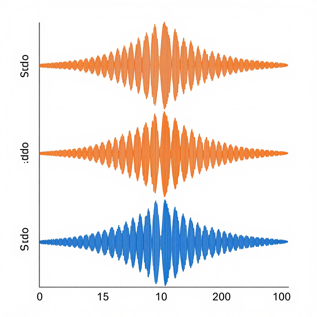
오디오 시각화
import matplotlib.pyplot as plt

# 파형 (Waveform)
fig, axes = plt.subplots(3, 1, figsize=(12, 8))

# 1. 시간 도메인 (파형)
time_axis = torch.arange(0, waveform.shape[1]) / sample_rate
axes[0].plot(time_axis, waveform[0])
axes[0].set_title("Waveform")
axes[0].set_xlabel("Time (s)")
axes[0].set_ylabel("Amplitude")

# 2. 스펙트로그램
spectrogram = torchaudio.transforms.Spectrogram(n_fft=1024)(waveform)
axes[1].imshow(
    spectrogram[0].log2().numpy(),
    aspect='auto', origin='lower', cmap='magma'
)
axes[1].set_title("Spectrogram")

# 3. Mel 스펙트로그램
mel_spec = torchaudio.transforms.MelSpectrogram(
    sample_rate=sample_rate, n_fft=1024, n_mels=80
)(waveform)
axes[2].imshow(
    mel_spec[0].log2().numpy(),
    aspect='auto', origin='lower', cmap='magma'
)
axes[2].set_title("Mel Spectrogram")

plt.tight_layout()
plt.savefig("audio_analysis.png", dpi=150)
Part 2: 핵심 변환 (Transforms)
스펙트로그램 계열
# STFT (Short-Time Fourier Transform)
# 시간 → 시간+주파수 영역으로 변환
spectrogram_transform = torchaudio.transforms.Spectrogram(
    n_fft=1024,       # FFT 윈도우 크기 (주파수 해상도)
    hop_length=256,    # 윈도우 이동 간격 (시간 해상도)
    win_length=1024,   # 윈도우 길이
    power=2.0,         # 2.0=파워, 1.0=진폭
)

spec = spectrogram_transform(waveform)
# shape: [channels, n_freq_bins, time_frames]
# n_freq_bins = n_fft // 2 + 1 = 513
n_fft와 hop_length의 트레이드오프:

n_fft ↑ → 주파수 해상도 ↑, 시간 해상도 ↓
n_fft ↓ → 주파수 해상도 ↓, 시간 해상도 ↑

일반적인 설정:
├── 음성: n_fft=400~512, hop=160 (16kHz 기준)
├── 음악: n_fft=2048, hop=512 (44.1kHz 기준)
└── 범용: n_fft=1024, hop=256
Mel 스펙트로그램 — 왜 Mel인가?
# 사람의 귀는 저주파에 민감, 고주파에 둔감
# Mel 스케일 = 인간 청각을 반영한 주파수 스케일

mel_transform = torchaudio.transforms.MelSpectrogram(
    sample_rate=16000,
    n_fft=1024,
    hop_length=256,
    n_mels=80,          # Mel 필터 개수 (보통 40~128)
    f_min=0,            # 최소 주파수
    f_max=8000,         # 최대 주파수 (Nyquist)
)

mel_spec = mel_transform(waveform)
# shape: [1, 80, time_frames]

# dB 스케일 변환 (로그 압축)
amplitude_to_db = torchaudio.transforms.AmplitudeToDB(stype='power', top_db=80)
mel_spec_db = amplitude_to_db(mel_spec)
Mel 주파수 변환 공식:
  mel = 2595 × log10(1 + freq / 700)

주파수 → Mel:
  100 Hz  →  150 mel   (저주파: 조밀)
  1000 Hz →  1000 mel
  4000 Hz →  2146 mel
  8000 Hz →  2840 mel  (고주파: 성긴)

→ 저주파는 세밀하게, 고주파는 뭉뚱그려서 분석
→ 사람이 듣는 것과 비슷한 표현!
MFCC (Mel-Frequency Cepstral Coefficients)
# MFCC = Mel 스펙트로그램 + DCT (이산 코사인 변환)
# 음성의 "형태"를 나타내는 핵심 특성

mfcc_transform = torchaudio.transforms.MFCC(
    sample_rate=16000,
    n_mfcc=13,          # MFCC 계수 개수 (보통 13~40)
    melkwargs={
        'n_fft': 1024,
        'n_mels': 80,
        'hop_length': 256,
    }
)

mfcc = mfcc_transform(waveform)
# shape: [1, 13, time_frames]

# Delta (1차 미분) + Delta-Delta (2차 미분)
# → 음성의 변화율 정보 추가
delta = torchaudio.functional.compute_deltas(mfcc)
delta_delta = torchaudio.functional.compute_deltas(delta)

# 최종 특성: [MFCC, Delta, Delta-Delta] 연결
features = torch.cat([mfcc, delta, delta_delta], dim=1)
# shape: [1, 39, time_frames]
어디에 쓰이나?
├── MFCC: 전통 음성인식 (HMM-GMM), 화자 인식
├── Mel Spectrogram: 딥러닝 음성인식 (Wav2Vec2, Whisper)
├── Spectrogram: 음악 분석, 환경음 분류
└── Raw Waveform: End-to-end 모델 (최신 트렌드)
Part 3: 오디오 Augmentation
# 시간 마스킹 (SpecAugment)
time_masking = torchaudio.transforms.TimeMasking(
    time_mask_param=30   # 최대 30 프레임 마스킹
)

# 주파수 마스킹 (SpecAugment)
freq_masking = torchaudio.transforms.FrequencyMasking(
    freq_mask_param=15   # 최대 15 채널 마스킹
)

# SpecAugment (음성인식 정확도 크게 향상!)
augmented_spec = time_masking(freq_masking(mel_spec))

# 시간 늘리기/줄이기
time_stretch = torchaudio.transforms.TimeStretch()
stretched = time_stretch(complex_spec, overriding_rate=1.2)  # 20% 빠르게

# 피치 변환
pitch_shift = torchaudio.transforms.PitchShift(
    sample_rate=16000, n_steps=4  # 4 반음 올리기
)
shifted = pitch_shift(waveform)

# 노이즈 추가
def add_noise(waveform, snr_db=10):
    """SNR dB 기준으로 백색 노이즈 추가"""
    noise = torch.randn_like(waveform)
    signal_power = waveform.norm(p=2)
    noise_power = noise.norm(p=2)
    snr = 10 ** (snr_db / 20)
    scale = signal_power / (snr * noise_power)
    return waveform + scale * noise
Part 4: 사전학습 모델
Wav2Vec 2.0 (음성인식)
import torchaudio
from torchaudio.pipelines import WAV2VEC2_ASR_BASE_960H

# 파이프라인 로드
bundle = WAV2VEC2_ASR_BASE_960H
model = bundle.get_model()
labels = bundle.get_labels()  # 토큰 목록

# 추론
waveform, sr = torchaudio.load("speech.wav")
if sr != bundle.sample_rate:
    waveform = torchaudio.transforms.Resample(sr, bundle.sample_rate)(waveform)

with torch.no_grad():
    emissions, _ = model(waveform)

# CTC 디코딩 (Greedy)
def greedy_decode(emissions, labels):
    indices = torch.argmax(emissions, dim=-1)[0]
    tokens = []
    prev = -1
    for idx in indices:
        if idx != prev and idx != 0:  # 0 = blank
            tokens.append(labels[idx])
        prev = idx
    return "".join(tokens).replace("|", " ").strip()

text = greedy_decode(emissions, labels)
print(f"인식 결과: {text}")
HuBERT (자기지도 음성 표현)
from torchaudio.pipelines import HUBERT_BASE

bundle = HUBERT_BASE
model = bundle.get_model()

with torch.no_grad():
    features, _ = model(waveform)
# features: [1, time_frames, 768]
# → 음성의 의미적 표현 벡터
# → 화자 인식, 감정 분석, 음성 분류에 활용
Forced Alignment (자막 동기화)
# 음성과 텍스트의 시간 정렬!
# → 자막 생성, 가사 동기화에 필수

from torchaudio.pipelines import MMS_FA  # Multilingual!

bundle = MMS_FA
model = bundle.get_model()
tokenizer = bundle.get_tokenizer()
aligner = bundle.get_aligner()

transcript = "안녕하세요 반갑습니다"
tokens = tokenizer(transcript)

with torch.no_grad():
    emissions, _ = model(waveform)

token_spans = aligner(emissions[0], tokens)
# 각 토큰의 시작/끝 시간을 프레임 단위로 반환!

for span, token in zip(token_spans, transcript):
    start_time = span.start * model.hop_length / sample_rate
    end_time = span.end * model.hop_length / sample_rate
    print(f"  '{token}': {start_time:.3f}s ~ {end_time:.3f}s")
Part 5: 오디오 이펙트
# torchaudio.functional — GPU 가속 오디오 처리

import torchaudio.functional as F

# 볼륨 조절
loud = F.gain(waveform, gain_db=6.0)    # +6dB
quiet = F.gain(waveform, gain_db=-6.0)  # -6dB

# 하이패스/로우패스 필터
highpass = F.highpass_biquad(waveform, sample_rate, cutoff_freq=300)
lowpass = F.lowpass_biquad(waveform, sample_rate, cutoff_freq=3000)

# 이퀄라이저
eq = F.equalizer_biquad(
    waveform, sample_rate,
    center_freq=1000,  # 1kHz 부근
    gain=5.0,          # +5dB 부스트
    Q=0.707
)

# 리버브 (잔향)
rir, _ = torchaudio.load("room_impulse_response.wav")  # RIR 파일
reverb = F.fftconvolve(waveform, rir)

# 페이드 인/아웃
fade = torchaudio.transforms.Fade(
    fade_in_len=sample_rate,      # 1초 페이드 인
    fade_out_len=sample_rate * 3  # 3초 페이드 아웃
)
faded = fade(waveform)

# VAD (Voice Activity Detection)
vad = torchaudio.transforms.Vad(sample_rate=16000)
speech_only = vad(waveform)  # 무음 구간 제거
Part 6: 실전 프로젝트
환경음 분류 (Audio Classification)
import torch.nn as nn

class AudioClassifier(nn.Module):
    def __init__(self, n_classes=10):
        super().__init__()
        self.mel = torchaudio.transforms.MelSpectrogram(
            sample_rate=16000, n_fft=1024, n_mels=64
        )
        self.db = torchaudio.transforms.AmplitudeToDB()

        # Mel 스펙트로그램을 "이미지"처럼 CNN에 입력!
        self.cnn = nn.Sequential(
            nn.Conv2d(1, 32, 3, padding=1), nn.ReLU(), nn.MaxPool2d(2),
            nn.Conv2d(32, 64, 3, padding=1), nn.ReLU(), nn.MaxPool2d(2),
            nn.Conv2d(64, 128, 3, padding=1), nn.ReLU(),
            nn.AdaptiveAvgPool2d((1, 1)),
        )
        self.fc = nn.Linear(128, n_classes)

    def forward(self, waveform):
        # [B, 1, samples] → [B, 1, n_mels, time]
        x = self.mel(waveform)
        x = self.db(x)
        x = self.cnn(x)
        x = x.view(x.size(0), -1)
        return self.fc(x)

# Mel 스펙트로그램 = 오디오의 "이미지"
# → CNN(ResNet, EfficientNet)으로 분류 가능!
실시간 스트리밍 처리
from torchaudio.io import StreamReader

# 마이크 입력 실시간 처리
reader = StreamReader(src=":0", format="avfoundation")  # macOS
reader.add_basic_audio_stream(
    frames_per_chunk=16000,  # 1초 단위
    sample_rate=16000,
)

for (chunk,) in reader.stream():
    # chunk: [1, 16000]
    mel = mel_transform(chunk)
    with torch.no_grad():
        prediction = model(mel)
    print(f"감지: {labels[prediction.argmax()]}")
📝 퀴즈 — torchaudio (클릭해서 확인!)
Q1. Mel 스케일이 필요한 이유는? ||인간의 청각은 저주파에 민감하고 고주파에 둔감. Mel 스케일은 이를 반영하여 저주파는 세밀하게, 고주파는 뭉뚱그려서 분석. 딥러닝 모델에 인간 청각 특성 반영||
Q2. n_fft를 키우면 어떤 해상도가 올라가고, 어떤 해상도가 내려가나? ||n_fft ↑ → 주파수 해상도 ↑ (세밀한 주파수 구분), 시간 해상도 ↓ (시간 변화 파악 어려움). 불확정성 원리와 유사한 트레이드오프||
Q3. SpecAugment의 두 가지 마스킹은? ||Time Masking: 시간 축에서 연속 프레임을 0으로 마스킹. Frequency Masking: 주파수 축에서 연속 채널을 0으로 마스킹. 데이터 augmentation으로 음성인식 정확도 크게 향상||
Q4. MFCC와 Mel Spectrogram의 차이와 각각의 용도는? ||MFCC: Mel Spectrogram에 DCT를 적용해 계수 추출 (13~40차원). 전통 음성인식, 화자 인식에 사용. Mel Spectrogram: 주파수-시간 2D 표현. 딥러닝 모델에 직접 입력 (최신 트렌드)||
Q5. Forced Alignment의 활용 사례는? ||음성과 텍스트의 시간 정렬. 자막 생성 (정확한 타이밍), 가사 동기화 (노래방), 발음 평가 (언어 학습 앱)||
Q6. Wav2Vec 2.0에서 CTC 디코딩의 blank 토큰 역할은? ||연속된 같은 토큰을 구분하고, 아무 출력도 없는 시간 구간을 표현. Greedy 디코딩에서 blank(index 0)과 연속 중복을 제거하여 최종 텍스트 생성||
Q7. Mel Spectrogram을 CNN에 넣을 수 있는 이유는? ||Mel Spectrogram은 2D 이미지와 같은 구조 (주파수 축 × 시간 축). 1채널 grayscale 이미지로 취급하여 ResNet, EfficientNet 등 이미지 분류 모델을 그대로 활용 가능||
📖 관련 시리즈 & 추천 포스팅
- torchvision 완전 가이드 — 이미지 AI (자매편)
- AI를 위한 수학 완전 가이드 — 푸리에 변환, 확률 (오디오 이해 필수)
- 나만의 GPT 만들기 — Wav2Vec2의 기반 Transformer
GitHub
- torchaudio 공식
- Whisper — OpenAI 음성인식
- ESPnet — 종합 음성처리 툴킷
The Complete torchaudio Guide — From Audio Processing to Speech Recognition, TTS, and Music Analysis
- Introduction
- Part 1: Audio Fundamentals
- Part 2: Core Transforms
- Part 3: Audio Augmentation
- Part 4: Pretrained Models
- Part 5: Audio Effects
- Part 6: Practical Projects
- Related Series and Recommended Posts
- Quiz
Introduction
torchaudio is the official audio processing library for PyTorch. It supports audio I/O, spectrogram transforms, pretrained models (Wav2Vec2, HuBERT, Whisper), and even real-time streaming.
pip install torch torchaudio
Part 1: Audio Fundamentals
Loading and Saving Audio
import torch
import torchaudio

# Load audio
waveform, sample_rate = torchaudio.load("speech.wav")
print(f"Shape: {waveform.shape}")    # [channels, samples]
print(f"Sample Rate: {sample_rate}")  # 16000
print(f"Duration: {waveform.shape[1] / sample_rate:.2f}s")

# Channels: mono (1) vs stereo (2)
if waveform.shape[0] == 2:
    mono = waveform.mean(dim=0, keepdim=True)  # Stereo -> Mono

# Resampling (44100Hz -> 16000Hz)
resampler = torchaudio.transforms.Resample(
    orig_freq=44100, new_freq=16000
)
waveform_16k = resampler(waveform)

# Save
torchaudio.save("output.wav", waveform_16k, 16000)

# Supported formats: wav, flac, mp3, ogg, opus, sphere
# Backends: sox, soundfile, ffmpeg
print(torchaudio.list_audio_backends())
Audio Visualization
import matplotlib.pyplot as plt

# Waveform
fig, axes = plt.subplots(3, 1, figsize=(12, 8))

# 1. Time domain (waveform)
time_axis = torch.arange(0, waveform.shape[1]) / sample_rate
axes[0].plot(time_axis, waveform[0])
axes[0].set_title("Waveform")
axes[0].set_xlabel("Time (s)")
axes[0].set_ylabel("Amplitude")

# 2. Spectrogram
spectrogram = torchaudio.transforms.Spectrogram(n_fft=1024)(waveform)
axes[1].imshow(
    spectrogram[0].log2().numpy(),
    aspect='auto', origin='lower', cmap='magma'
)
axes[1].set_title("Spectrogram")

# 3. Mel Spectrogram
mel_spec = torchaudio.transforms.MelSpectrogram(
    sample_rate=sample_rate, n_fft=1024, n_mels=80
)(waveform)
axes[2].imshow(
    mel_spec[0].log2().numpy(),
    aspect='auto', origin='lower', cmap='magma'
)
axes[2].set_title("Mel Spectrogram")

plt.tight_layout()
plt.savefig("audio_analysis.png", dpi=150)
Part 2: Core Transforms
Spectrogram Family
# STFT (Short-Time Fourier Transform)
# Converts from time domain to time+frequency domain
spectrogram_transform = torchaudio.transforms.Spectrogram(
    n_fft=1024,       # FFT window size (frequency resolution)
    hop_length=256,    # Window hop interval (time resolution)
    win_length=1024,   # Window length
    power=2.0,         # 2.0=power, 1.0=amplitude
)

spec = spectrogram_transform(waveform)
# shape: [channels, n_freq_bins, time_frames]
# n_freq_bins = n_fft // 2 + 1 = 513
Trade-off between n_fft and hop_length:

n_fft up -> frequency resolution up, time resolution down
n_fft down -> frequency resolution down, time resolution up

Common settings:
+-- Speech: n_fft=400~512, hop=160 (at 16kHz)
+-- Music: n_fft=2048, hop=512 (at 44.1kHz)
+-- General: n_fft=1024, hop=256
Mel Spectrogram — Why Mel?
# The human ear is sensitive to low frequencies, less so to high frequencies.
# Mel scale = a frequency scale that reflects human auditory perception.

mel_transform = torchaudio.transforms.MelSpectrogram(
    sample_rate=16000,
    n_fft=1024,
    hop_length=256,
    n_mels=80,          # Number of Mel filters (typically 40~128)
    f_min=0,            # Minimum frequency
    f_max=8000,         # Maximum frequency (Nyquist)
)

mel_spec = mel_transform(waveform)
# shape: [1, 80, time_frames]

# Convert to dB scale (log compression)
amplitude_to_db = torchaudio.transforms.AmplitudeToDB(stype='power', top_db=80)
mel_spec_db = amplitude_to_db(mel_spec)
Mel frequency conversion formula:
  mel = 2595 * log10(1 + freq / 700)

Frequency -> Mel:
  100 Hz  ->  150 mel   (low freq: dense)
  1000 Hz ->  1000 mel
  4000 Hz ->  2146 mel
  8000 Hz ->  2840 mel  (high freq: sparse)

-> Low frequencies are analyzed finely, high frequencies are coarsely grouped
-> A representation similar to how humans hear!
MFCC (Mel-Frequency Cepstral Coefficients)
# MFCC = Mel Spectrogram + DCT (Discrete Cosine Transform)
# Key features representing the "shape" of speech

mfcc_transform = torchaudio.transforms.MFCC(
    sample_rate=16000,
    n_mfcc=13,          # Number of MFCC coefficients (typically 13~40)
    melkwargs={
        'n_fft': 1024,
        'n_mels': 80,
        'hop_length': 256,
    }
)

mfcc = mfcc_transform(waveform)
# shape: [1, 13, time_frames]

# Delta (1st derivative) + Delta-Delta (2nd derivative)
# -> Adds rate-of-change information for speech
delta = torchaudio.functional.compute_deltas(mfcc)
delta_delta = torchaudio.functional.compute_deltas(delta)

# Final features: concatenate [MFCC, Delta, Delta-Delta]
features = torch.cat([mfcc, delta, delta_delta], dim=1)
# shape: [1, 39, time_frames]
Where are these used?
+-- MFCC: Traditional speech recognition (HMM-GMM), speaker recognition
+-- Mel Spectrogram: Deep learning speech recognition (Wav2Vec2, Whisper)
+-- Spectrogram: Music analysis, environmental sound classification
+-- Raw Waveform: End-to-end models (latest trend)
Part 3: Audio Augmentation
# Time masking (SpecAugment)
time_masking = torchaudio.transforms.TimeMasking(
    time_mask_param=30   # Mask up to 30 frames
)

# Frequency masking (SpecAugment)
freq_masking = torchaudio.transforms.FrequencyMasking(
    freq_mask_param=15   # Mask up to 15 channels
)

# SpecAugment (significantly improves speech recognition accuracy!)
augmented_spec = time_masking(freq_masking(mel_spec))

# Time stretching
time_stretch = torchaudio.transforms.TimeStretch()
stretched = time_stretch(complex_spec, overriding_rate=1.2)  # 20% faster

# Pitch shifting
pitch_shift = torchaudio.transforms.PitchShift(
    sample_rate=16000, n_steps=4  # Shift up by 4 semitones
)
shifted = pitch_shift(waveform)

# Adding noise
def add_noise(waveform, snr_db=10):
    """Add white noise based on SNR in dB"""
    noise = torch.randn_like(waveform)
    signal_power = waveform.norm(p=2)
    noise_power = noise.norm(p=2)
    snr = 10 ** (snr_db / 20)
    scale = signal_power / (snr * noise_power)
    return waveform + scale * noise
Part 4: Pretrained Models
Wav2Vec 2.0 (Speech Recognition)
import torchaudio
from torchaudio.pipelines import WAV2VEC2_ASR_BASE_960H

# Load pipeline
bundle = WAV2VEC2_ASR_BASE_960H
model = bundle.get_model()
labels = bundle.get_labels()  # Token list

# Inference
waveform, sr = torchaudio.load("speech.wav")
if sr != bundle.sample_rate:
    waveform = torchaudio.transforms.Resample(sr, bundle.sample_rate)(waveform)

with torch.no_grad():
    emissions, _ = model(waveform)

# CTC Decoding (Greedy)
def greedy_decode(emissions, labels):
    indices = torch.argmax(emissions, dim=-1)[0]
    tokens = []
    prev = -1
    for idx in indices:
        if idx != prev and idx != 0:  # 0 = blank
            tokens.append(labels[idx])
        prev = idx
    return "".join(tokens).replace("|", " ").strip()

text = greedy_decode(emissions, labels)
print(f"Recognition result: {text}")
HuBERT (Self-Supervised Speech Representations)
from torchaudio.pipelines import HUBERT_BASE

bundle = HUBERT_BASE
model = bundle.get_model()

with torch.no_grad():
    features, _ = model(waveform)
# features: [1, time_frames, 768]
# -> Semantic representation vectors of speech
# -> Used for speaker recognition, emotion analysis, speech classification
Forced Alignment (Subtitle Synchronization)
# Temporal alignment between speech and text!
# -> Essential for subtitle generation and lyrics synchronization

from torchaudio.pipelines import MMS_FA  # Multilingual!

bundle = MMS_FA
model = bundle.get_model()
tokenizer = bundle.get_tokenizer()
aligner = bundle.get_aligner()

transcript = "hello nice to meet you"
tokens = tokenizer(transcript)

with torch.no_grad():
    emissions, _ = model(waveform)

token_spans = aligner(emissions[0], tokens)
# Returns start/end times for each token in frame units!

for span, token in zip(token_spans, transcript):
    start_time = span.start * model.hop_length / sample_rate
    end_time = span.end * model.hop_length / sample_rate
    print(f"  '{token}': {start_time:.3f}s ~ {end_time:.3f}s")
Part 5: Audio Effects
# torchaudio.functional — GPU-accelerated audio processing

import torchaudio.functional as F

# Volume adjustment
loud = F.gain(waveform, gain_db=6.0)    # +6dB
quiet = F.gain(waveform, gain_db=-6.0)  # -6dB

# High-pass / Low-pass filter
highpass = F.highpass_biquad(waveform, sample_rate, cutoff_freq=300)
lowpass = F.lowpass_biquad(waveform, sample_rate, cutoff_freq=3000)

# Equalizer
eq = F.equalizer_biquad(
    waveform, sample_rate,
    center_freq=1000,  # Around 1kHz
    gain=5.0,          # +5dB boost
    Q=0.707
)

# Reverb
rir, _ = torchaudio.load("room_impulse_response.wav")  # RIR file
reverb = F.fftconvolve(waveform, rir)

# Fade in/out
fade = torchaudio.transforms.Fade(
    fade_in_len=sample_rate,      # 1 second fade in
    fade_out_len=sample_rate * 3  # 3 second fade out
)
faded = fade(waveform)

# VAD (Voice Activity Detection)
vad = torchaudio.transforms.Vad(sample_rate=16000)
speech_only = vad(waveform)  # Remove silent segments
Part 6: Practical Projects
Environmental Sound Classification (Audio Classification)
import torch.nn as nn

class AudioClassifier(nn.Module):
    def __init__(self, n_classes=10):
        super().__init__()
        self.mel = torchaudio.transforms.MelSpectrogram(
            sample_rate=16000, n_fft=1024, n_mels=64
        )
        self.db = torchaudio.transforms.AmplitudeToDB()

        # Feed the Mel spectrogram into a CNN as if it were an "image"!
        self.cnn = nn.Sequential(
            nn.Conv2d(1, 32, 3, padding=1), nn.ReLU(), nn.MaxPool2d(2),
            nn.Conv2d(32, 64, 3, padding=1), nn.ReLU(), nn.MaxPool2d(2),
            nn.Conv2d(64, 128, 3, padding=1), nn.ReLU(),
            nn.AdaptiveAvgPool2d((1, 1)),
        )
        self.fc = nn.Linear(128, n_classes)

    def forward(self, waveform):
        # [B, 1, samples] -> [B, 1, n_mels, time]
        x = self.mel(waveform)
        x = self.db(x)
        x = self.cnn(x)
        x = x.view(x.size(0), -1)
        return self.fc(x)

# Mel Spectrogram = an "image" of audio
# -> Can be classified with CNNs (ResNet, EfficientNet)!
Real-Time Streaming Processing
from torchaudio.io import StreamReader

# Real-time microphone input processing
reader = StreamReader(src=":0", format="avfoundation")  # macOS
reader.add_basic_audio_stream(
    frames_per_chunk=16000,  # 1 second chunks
    sample_rate=16000,
)

for (chunk,) in reader.stream():
    # chunk: [1, 16000]
    mel = mel_transform(chunk)
    with torch.no_grad():
        prediction = model(mel)
    print(f"Detected: {labels[prediction.argmax()]}")
Quiz — torchaudio (click to reveal!)
Q1. Why is the Mel scale needed? ||Human hearing is sensitive to low frequencies and less responsive to high frequencies. The Mel scale reflects this by analyzing low frequencies finely and grouping high frequencies coarsely. It incorporates human auditory characteristics into deep learning models.||
Q2. When you increase n_fft, which resolution goes up and which goes down? ||n_fft up -> frequency resolution up (finer frequency discrimination), time resolution down (harder to track temporal changes). A trade-off similar to the uncertainty principle.||
Q3. What are the two types of masking in SpecAugment? ||Time Masking: masks consecutive frames along the time axis with zeros. Frequency Masking: masks consecutive channels along the frequency axis with zeros. As data augmentation, these significantly improve speech recognition accuracy.||
Q4. What is the difference between MFCC and Mel Spectrogram, and what are their use cases? ||MFCC: Applies DCT to Mel Spectrogram to extract coefficients (13~40 dimensions). Used in traditional speech recognition and speaker recognition. Mel Spectrogram: A 2D time-frequency representation. Fed directly into deep learning models (current trend).||
Q5. What are the applications of Forced Alignment? ||Temporal alignment of speech and text. Subtitle generation (accurate timing), lyrics synchronization (karaoke), pronunciation assessment (language learning apps).||
Q6. What role does the blank token play in CTC decoding for Wav2Vec 2.0? ||It separates consecutive identical tokens and represents time intervals with no output. In greedy decoding, blanks (index 0) and consecutive duplicates are removed to produce the final text.||
Q7. Why can a Mel Spectrogram be fed into a CNN? ||A Mel Spectrogram has the same structure as a 2D image (frequency axis x time axis). It can be treated as a 1-channel grayscale image, allowing direct use of image classification models like ResNet and EfficientNet.||
Related Series and Recommended Posts
- The Complete torchvision Guide — Image AI (companion post)
- The Complete Math for AI Guide — Fourier Transform, Probability (essential for understanding audio)
- Build Your Own GPT — The Transformer behind Wav2Vec2
GitHub
- torchaudio Official
- Whisper — OpenAI Speech Recognition
- ESPnet — Comprehensive Speech Processing Toolkit
Quiz
Q1: What is the main topic covered in "The Complete torchaudio Guide — From Audio Processing to
Speech Recognition, TTS, and Music Analysis"?
From audio loading and spectrogram transforms to Mel filter banks, MFCC, speech recognition (Wav2Vec2/Whisper), TTS, speaker diarization, and noise reduction — everything about audio AI with PyTorch.
Q2: What is Part 1: Audio Fundamentals?
Loading and Saving Audio Audio Visualization
Q3: Explain the core concept of Part 2: Core Transforms.
Spectrogram Family Mel Spectrogram — Why Mel? MFCC (Mel-Frequency Cepstral Coefficients)
Q4: What are the key aspects of Part 4: Pretrained Models?
Wav2Vec 2.0 (Speech Recognition) HuBERT (Self-Supervised Speech Representations) Forced Alignment
(Subtitle Synchronization)
Q5: How does Part 6: Practical Projects work?
Environmental Sound Classification (Audio Classification) Real-Time Streaming Processing Q1. Why
is the Mel scale needed? Q2. When you increase n_fft, which resolution goes up and which goes
down? Q3. What are the two types of masking in SpecAugment? Q4.